In this blog post, we’ll explore several algorithms to cluster data points.

Some notation:

• Boldface capital letters like $\mathbf{A}$ are matrices.
• Boldface lowercase letters like $\mathbf{v}$ are vectors.

The clustering problem

We’re aiming to solve the problem of assigning labels to observations based on the distribution of their features. In this exercise, the features are represented as the matrix $\mathbf{X}$, with each row representing a data point and each data point being in $\mathbb{R}^2$. We are also dealing with the simple case of 2 clusters for now. What we do generalize is the shape of the distribution in $\mathbb{R}^2$. But first, let’s look at a simple 2-cluster distribution.

import numpy as np
from sklearn import datasets
from matplotlib import pyplot as plt

n = 200
np.random.seed(1111)
X, y = datasets.make_blobs(n_samples=n, shuffle=True, random_state=None, centers = 2, cluster_std = 2.0)
plt.scatter(X[:,0], X[:,1])

<matplotlib.collections.PathCollection at 0x7fbfd8bea580>

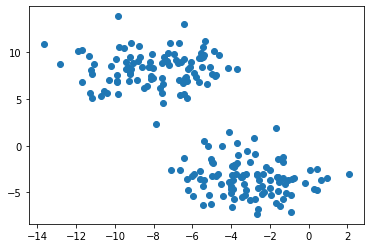
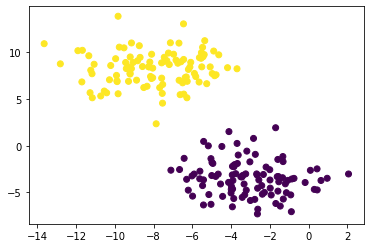
For this simple distribution, we can use k-means clustering. Intuitively, this minimizes the distances between each cluster’s members and its “center of gravity”, and works well for roughly circular blobs.

from sklearn.cluster import KMeans
km = KMeans(n_clusters = 2)
km.fit(X)

plt.scatter(X[:,0], X[:,1], c = km.predict(X))

Generalizing the distribution

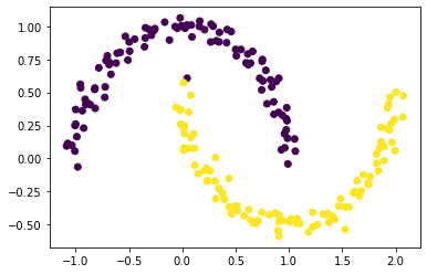
Now let’s look at this distribution of data points.

np.random.seed(1234)
n = 200
X, y = datasets.make_moons(n_samples=n, shuffle=True, noise=0.05, random_state=None)
plt.scatter(X[:,0], X[:,1])

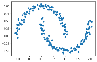
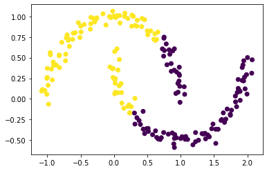
The two clusters are still obvious by sight, but k-means clustering fails.

km = KMeans(n_clusters = 2)
km.fit(X)
plt.scatter(X[:,0], X[:,1], c = km.predict(X))

Constructing a similarity matrix A

An important ingredient in all of the clustering algorithms in this post is the similarity matrix similarity matrix $\mathbf{A}$. A is a symmetric square matrix with n rows and columns. A[i,j] should be equal to 1 if and only if X[i] is close to X[j]. To quantify closeness, we will have a threshold distance epsilon, set to 0.4 for now. The diagonal entries A[i,i] should all be equal to zero.

from sklearn.metrics import pairwise_distances

epsilon = 0.4

dist = pairwise_distances(X)
A = np.array(dist < epsilon).astype('int')
np.fill_diagonal(A,0)

A

array([[0, 0, 0, ..., 0, 0, 0],
       [0, 0, 0, ..., 0, 0, 0],
       [0, 0, 0, ..., 0, 1, 0],
       ...,
       [0, 0, 0, ..., 0, 1, 1],
       [0, 0, 1, ..., 1, 0, 1],
       [0, 0, 0, ..., 1, 1, 0]])

Norm cut objective function

Now that we have encoded the pairwise distances of the data points in $\mathbf{A}$, we can define the clustering problem as a minimization problem. Intuitively, the parameter space of this minimization problem should be the possible cluster assignments (a vector of n 0s and 1s), and the objective function should decrease when our assignment yields more proximity within each cluster, and increase when our assignment yields more proximity between different clusters.

We thus define the binary norm cut objective of the similarity matrix $\mathbf{A}$ :

In this expression,

• $C_0$ and $C_1$ are the clusters assigned.
• $\mathbf{cut}(C_0, C_1) \equiv \sum_{i \in C_0, j \in C_1} a_{ij}$ (the “cut”) is the number of ones in $\mathbf{A}$ connecting $C_0$ to cluster $C_1$.
• $\mathbf{vol}(C_0) \equiv \sum_{i \in C_0}d_i$, where $d_i = \sum_{j = 1}^n a_{ij}$ is the degree of row $i$. This volume term measures the size and connectedness within the closter $C_0$.

The cut term

The function cut(A,y) below computes the cut term. We first construct a diff matrix ($n$ by $n$), whose $i,j$-th term is an indicator for points i and j being in different clusters under classification y. We then elementwise-multiply it with the similarity matrix.

def cut(A,y):
    # diff[i,j] is 1 iff y[i] is in a different group than y[j]
    diff = np.array([y != i for i in y], dtype='int')
    # return sum of entries in A where diff is 1, divide by 2 due to double counting
    return np.sum(np.multiply(diff,A))/2

We first test it with the true labels, y.

cut(A,y)

13.0

…and then with randomly generated labels

randn = np.random.randint(0,2,n)
cut(A,randn)

1150.0

As expected, the true labels yield a lower cut term than the fake labels.

The Volume Term

Now we compute the volume of each cluster. The volume of the cluster is just the sum of degrees of the cluster’s elements. Remember we want to minimize $\frac{1}{\mathbf{vol}(C_0)}$ so we want to maximize the volume.

def vols(A,y):
    # sum the rows of A where the row belongs to the cluster
    v0 = np.sum(A[y==0,])
    v1 = np.sum(A[y==1,])
    return v0, v1

Now we have all the ingredients for the norm cut objective.

def normcut(A,y):
    v0, v1 = vols(A,y)
    return cut(A,y) * (1/v0 + 1/v1)

print(vols(A,y))
print(normcut(A,y))

(2299, 2217)
0.011518412331615225

Again, the true labels y yield a much lower minimizing value than the random labels.

normcut(A,randn)

1.0240023597759158

Part C

Unfortunately, with what we have, the parameter space (the possible set of labels) is too large for a computationally efficient algorithm. This is why we need some linear algebra magic to give us another formula for the norm cut objective:

where

• $\mathbf{D}$ is the diagonal matrix with nonzero entries $d_{ii} = d_i$, and where $d_i = \sum_{j = 1}^n a_i$ is the degree.
• and $\mathbf{z}$ is a vector such that \(z_i = \begin{cases} \frac{1}{\mathbf{vol}(C_0)} &\quad \text{if } y_i = 0 \\ -\frac{1}{\mathbf{vol}(C_1)} &\quad \text{if } y_i = 1 \\ \end{cases}\)

Since the volume term is just a function of A and y, $\mathbf{z}$ encodes all the information in A and y through the volume term and the sign. We define the function transform(A,y) to compute the appropriate $\mathbf{z}$ vector.

def transform(A,y):
    # compute volumes
    v0, v1 = vols(A,y)
    # initialize z to be array of same shape as y, then fill depending on y
    z = np.where(y==0, 1/v0, -1/v1)
    return z

z = transform(A,y)
# degree matrix: row sums placed on diagonal
# the "at" sign is the matrix product
D = np.diag(A@np.ones(n))
normcut_formula = (z@(D-A)@z)/(z@D@z)
normcut_formula

0.011518412331615099

We check that the value of the norm cut function is numerically close by either method.

np.isclose(normcut(A,y), normcut_formula)

True

We can also check the identity $\mathbf{z}^T\mathbf{D}\mathbb{1} = 0$, where $\mathbb{1}$ is the vector of n ones. This identity effectively says that $\mathbf{z}$ should contain roughly as many positive as negative entries, i.e. as many labels in each cluster.

D = np.diag(A@np.ones(n))
np.isclose((z@D@np.ones(n)),0)

True

We denote the objective function

We can minimize this function subject to the condition $\mathbf{z}^T\mathbf{D}\mathbb{1} = 0$, which says that the clusters ar equally sized. We can guarantee the condition holds if, instead of minimizing over $\mathbf{z}$, we minimize the orthogonal complement of $\mathbf{z}$ relative to $\mathbf{D}\mathbb{1}$. The orth_obj function computes this. Then we use the minimize function from scipy.optimize to minimize the function orth_obj with respect to $\mathbf{z}$.

def orth(u, v):
    return (u @ v) / (v @ v) * v

e = np.ones(n)

d = D @ e

def orth_obj(z):
    z_o = z - orth(z, d)
    return (z_o @ (D - A) @ z_o)/(z_o @ D @ z_o)

from scipy.optimize import minimize

z_min = minimize(fun=orth_obj, x0=np.ones(n)).x

By construction, the sign of z_min[i] corresponds to the cluster label of data point i. We plot the points below, coloring it by the sign of z_min.

plt.scatter(X[:,0], X[:,1], c = (z_min >= 0))

Part F

Explicitly minimizing the orthogonal objective is extremely slow, but thankfully find a solution using eigenvalues and eigenvectors.

The Rayleigh-Ritz Theorem implies that the minimizing $\mathbf{z}$ is a solution to the eigenvalue problem

Since $\mathbb{1}$ is the eigenvector with smallest eigenvalue, the vector $\mathbf{z}$ that we want must be the eigenvector with the second-smallest eigenvalue.

We construct the Laplacian matrix of $\mathbf{A}$, $\mathbf{L} = \mathbf{D}^{-1}(\mathbf{D} - \mathbf{A})$, and find the eigenvector corresponding to its second-smallest eigenvalue, z_eig.

L = np.linalg.inv(D)@(D-A)

Lam, U = np.linalg.eig(L)
z_eig = U[:,1]

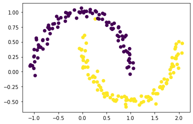
Now we color the point according to the sign of z_eig. Looks pretty good.

plt.scatter(X[:,0], X[:,1], c = z_eig<0)

Finally, we can define spectral_clustering(X, epsilon) which takes in the input data X and the distance threshold epsilon, performs spectral clustering, and returns an array of labels indicating whether data point i is in group 0 or group 1.

def spectral_clustering(X, epsilon):
    '''
    Given input X (n by 2 array) and distance threshold epsilon,
    performs spectral clustering, and
    returns n by 1 labels of cluster classification.
    '''
    A = np.array(pairwise_distances(X) < epsilon).astype('int')
    np.fill_diagonal(A,0)
    D = np.diag(A@np.ones(X.shape[0]))
    L = np.linalg.inv(D)@(D-A)
    Lam, U = np.linalg.eig(L)
    z_eig = U[:,1]
    labels = np.array(z_eig<0, dtype='int')
    return labels

spectral_clustering(X,0.4)

array([1, 1, 0, 0, 0, 0, 0, 0, 1, 1, 1, 0, 0, 1, 1, 1, 1, 0, 0, 0, 1, 1,
       1, 0, 0, 1, 0, 1, 1, 0, 0, 1, 1, 1, 1, 1, 0, 1, 1, 0, 1, 0, 0, 0,
       0, 0, 0, 1, 1, 1, 0, 0, 1, 1, 0, 0, 1, 1, 1, 0, 0, 0, 1, 0, 1, 0,
       0, 0, 0, 1, 1, 1, 1, 0, 0, 0, 1, 0, 1, 0, 0, 0, 0, 1, 1, 1, 1, 0,
       0, 0, 0, 1, 0, 0, 1, 1, 1, 1, 0, 0, 1, 1, 1, 0, 1, 1, 0, 0, 1, 1,
       0, 0, 0, 1, 0, 0, 0, 0, 1, 1, 1, 0, 1, 1, 1, 0, 1, 0, 1, 1, 0, 0,
       0, 0, 1, 1, 1, 1, 1, 1, 1, 1, 0, 0, 1, 0, 0, 0, 0, 0, 0, 0, 0, 1,
       1, 0, 1, 0, 0, 0, 1, 1, 0, 0, 1, 1, 1, 0, 0, 0, 1, 0, 1, 1, 1, 0,
       0, 0, 0, 1, 1, 0, 0, 1, 1, 1, 0, 1, 1, 1, 0, 1, 0, 1, 1, 1, 1, 0,
       0, 0])

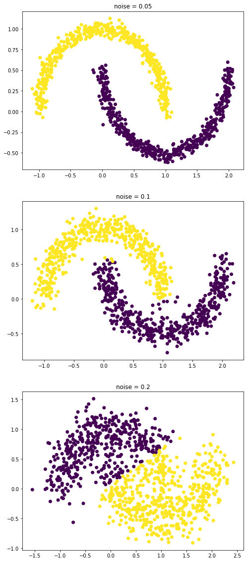
Now we can run som experiments, making the problem harder by increasing the noise parameter, and increase the computation by increasing n.

np.random.seed(123)
fig, axs = plt.subplots(3, figsize = (8,20))
noises = [0.05, 0.1, 0.2]
for i in range(3):
    X, y = datasets.make_moons(n_samples=1000, shuffle=True, noise=noises[i], random_state=None)
    axs[i].scatter(X[:,0], X[:,1], c = spectral_clustering(X,0.4))
    axs[i].set_title(label = "noise = " + str(noises[i]))

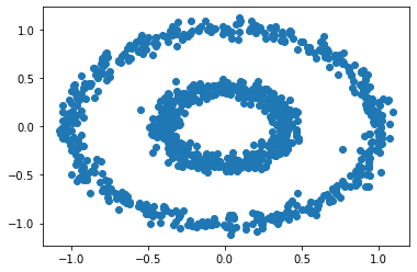
How does it perform on a different distribution?

n = 1000
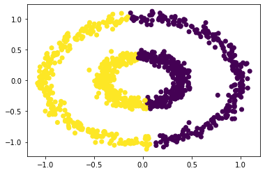
X, y = datasets.make_circles(n_samples=n, shuffle=True, noise=0.05, random_state=None, factor = 0.4)
plt.scatter(X[:,0], X[:,1])

# k-means fails
km = KMeans(n_clusters = 2)
km.fit(X)
plt.scatter(X[:,0], X[:,1], c = km.predict(X))

By adjusting the distance parameter epsilon, we can find a way to cluster the two circular blobs. We do run into singularity issues for some values of epsilon, but otherwise the results are plotted below.

fig, axs = plt.subplots(11, figsize=(8,50))
for i in range(3,11):
    epsilon = i/10
    try:
        axs[i].scatter(X[:,0], X[:,1], c = spectral_clustering(X,epsilon))
        axs[i].set_title(label = "epsilon = " + str(epsilon))
    except:
        print("Error when epsilon = ", epsilon)

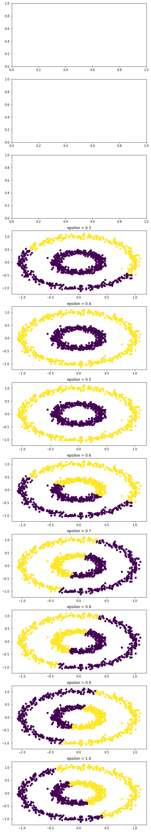
epsilon = 0.4 and 0.5 both work for this particular dataset.